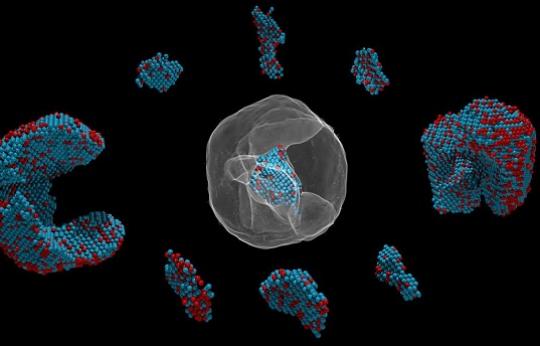
Traditionally image denoising in electron and X-ray microscopy relies on subtracting a background that is either a constant throughout the image, or by mathematically estimating a smooth background using methods such as the Laplace’s equation. Such methods are either too crude, or required segmenting the object and creating a mask in order to form the boundary for estimation, and also oftentimes requires manually-chosen tuning parameters for optimal performance. Here, I played around with a deep learning approach to denoising electron microscopy images, where I trained a CNN to recognize and subtract out artifacts in noisy tomography projection images to recover images that are more faithful to the true objects.

Tomography, or 3D imaging, aims to reconstruct a 3D representation of an object based on a series of 2D projections. This is the principle behind CT scans that you see in hospitals. Experimentally, projections are acquired by tilting the camera or the sample with respect to each other. When imaging objects on the nanoscale, undesirable background often reduces the quality of reconstruction. Therefore, background subtraction is a necessary step of projection preprocessing since tomography assumes the object to be isolated. So the question is this: given a series of tomography projection images corrupted by unwanted background, is it possible to train a CNN to subtract the background from the object of interest?

import numpy as np
import matplotlib.pyplot as plt
import pandas as pd
import scipy.io as sio
from scipy.ndimage.filters import gaussian_filter
import cv2
import glob
%matplotlib inline

Analytics approach

• Use a feed-forward denoising convolutional neural networks (DnCNN) backbone to train a model to recognize background in atomic electron tomography (AET) projection images
• DnCNN implicitly removes the latent clean image with the operations in the hidden layers. It uses residual learning and batch normalization (normalizes output of previous activation layer by subtracting the batch mean and dividing by the batch standard deviation) to speed up the training process as well as boost the denoising performance.
• Residual learning is used since residual image is easier to be learned than the original unreferenced mapping in a very deep neural network
• Image formation forward model follows this image degradation model: \(y = x + N\) Where \(y\) is the measured image, \(x\) is the uncorrupted true image, and \(N\) is artifact, or in this case, unwanted background. DnCNN attempts to fnd \(N\) and subtract from \(x\).

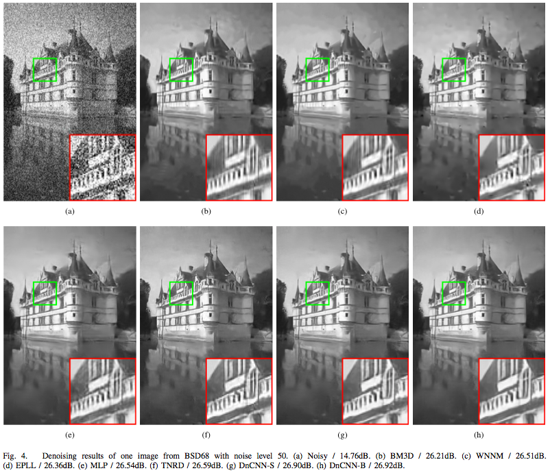
DnCNN architecture consists of one convolution + ReLu layer followed by 15 layers of layer of convolution + batch normalization + ReLu layers, followed by one layer of convolution. For natural images, it produces results like those seen below.

Data understanding

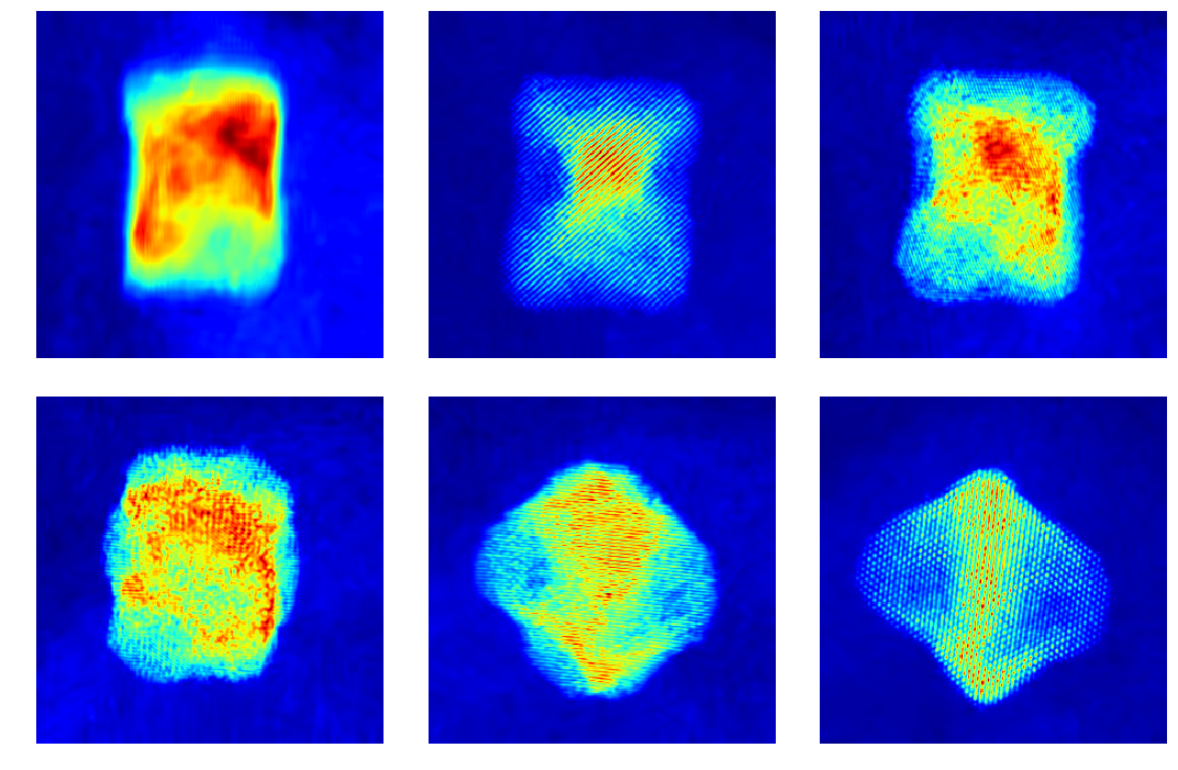
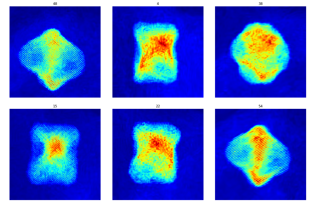
To understand what background in actual experimental data looks like, let’s check some raw projection tilt series. Notice that the background is mostly smooth and uneven, with varying intensities and distributions between them.

test_raw = sio.loadmat('./data_aet/Raw/NiPt_Mo_FS_171118_t2_BM3D100_results.mat')
test_raw = test_raw['Dset']
plt.figure(figsize=(15,10))
c = 1
for i in range(1, 60, 10):
    plt.subplot(2,3,c)
    plt.imshow(test_raw[:,:,i], cmap='jet')
    plt.axis('off')
    plt.tight_layout()
    c += 1    

Data requirements and collection

To acquire training data to train the model, multislice wave propagation method was used to simulate realistic STEM projection tilt series based on known atomic coordinates and elemental species. In this case parameters for nickel platinum is used. The simulated tilt series without background look like this:

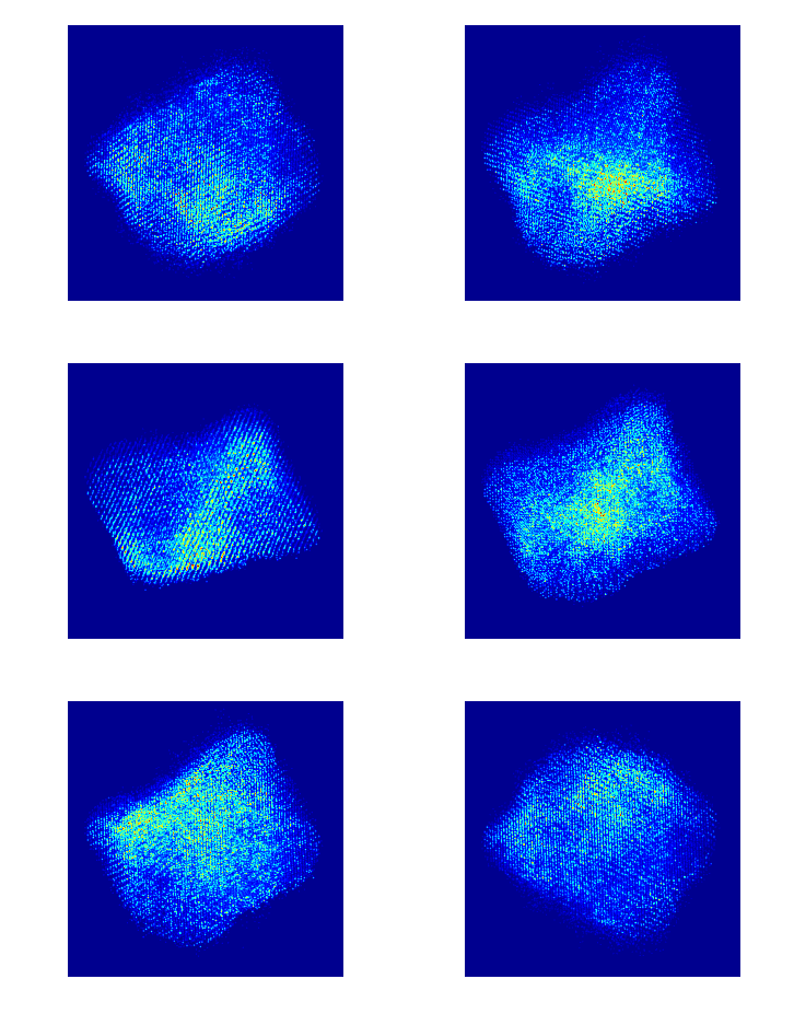
Each individual dot represents the electron density from an individual atom. In this particle there are more than 10,000 atoms.

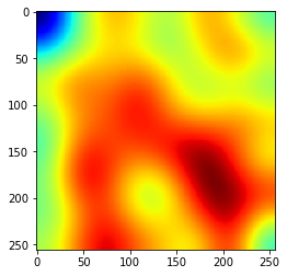
The smooth background was then simulated as Gaussian-smoothed random image, as seen below.

def gen_nubg(w, h, z): 
    '''generate non-uniform backgrounds (nuBG) for AET BG estimation'''
    background = np.zeros((w, h, z))
    for i in range(z):
        F = np.random.randint(10, 30)
        background[:,:,i] = gaussian_filter(np.random.randn(w, h), F)
    return background

background = gen_nubg(256, 256, 1)
plt.imshow(np.squeeze(background), cmap='jet');

Data preparation

• The training images (clean+background) are augmented (flipped up-down and rotated by 90 degrees) to generate more training data and
• Divided into 215,460 patches, each 40x40 in size, for faster and more effective training

Below you can see an example patch.

aet_patch = np.load('./data_aet/Train/npy_data/clean_patches.npy')
bg_patch = np.load('./data_aet/Train/npy_data/nu_backgrounds.npy')
print(aet_patch.shape)
print(bg_patch.shape)

idx = 21000

fig, ax = plt.subplots(nrows=1, ncols=3, figsize=(17, 4))
f1 = ax[0].imshow(np.squeeze(bg_patch[idx,:,:]), cmap='jet')
ax[0].title.set_text('Background')
fig.colorbar(f1, ax=ax[0])
f2 = ax[1].imshow(np.squeeze(aet_patch[idx,:,:]), cmap='jet')
fig.colorbar(f2, ax=ax[1])
ax[1].title.set_text('Clean image')
f3 = ax[2].imshow(np.squeeze(aet_patch[idx,:,:]) + np.squeeze(bg_patch[idx,:,:]), cmap='jet')
fig.colorbar(f3, ax=ax[2])
ax[2].title.set_text('Corrupt')

(215460, 40, 40)
(215460, 40, 40)

Modeling

For training the network:

• Training data is divided into 90%-10% training (162) and validation (18) split
• Uses TF-Keras implementation of DnCNN
• Optimizer: Adam
• Learning rate: 1e-3
• Error metric: mean square error
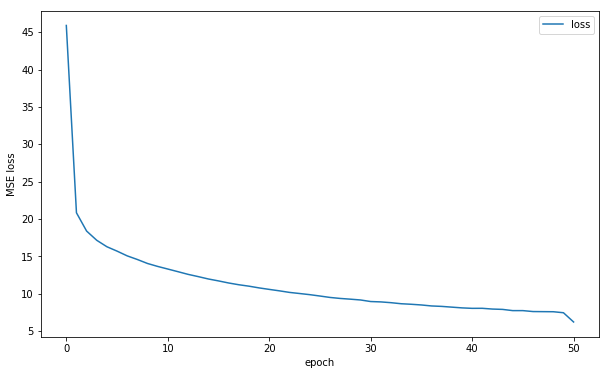
• Epoch: 51
• Training time: ~12 hours on Nvidia P4 GPU (computer clusters)
• Also calculated SSIM and PSNR

Training error is shown below. More epochs can improve performance as it does not seem to have converged yet.

df = pd.read_csv('./snapshot/save_DnCNN_sigma25_2019-08-28-15-32-13/log.csv')
ax_df = df.plot(x='epoch', y='loss', figsize=(10,6))
ax_df.set_ylabel('MSE loss');

Validation results

fnames = glob.glob('./results/val/*.mat')
iid = 13

for i in [iid]:
    f = sio.loadmat(fnames[i])
    fig, ax = plt.subplots(nrows=1, ncols=3, figsize=(17, 4))
    f1 = ax[0].imshow(np.squeeze(f['clean_img']), cmap='jet')
    fig.colorbar(f1, ax=ax[0])
    ax[0].title.set_text('Clean')
    f2 = ax[1].imshow(np.squeeze(f['test_img']), cmap='jet')
    fig.colorbar(f2, ax=ax[1])
    ax[1].title.set_text('Corrupt')
    f3 = ax[2].imshow(np.squeeze(f['out_img']), cmap='jet')
    fig.colorbar(f3, ax=ax[2])
    ax[2].title.set_text('Processed')

df2 = pd.read_csv('./results/val/metrics.csv')
df2.mean()

Unnamed: 0     9.000000
psnr          42.316029
ssim           0.990934
dtype: float64

SSIM of processed image is very high, suggesting background subtraction was successful.

Evaluation on experimental data

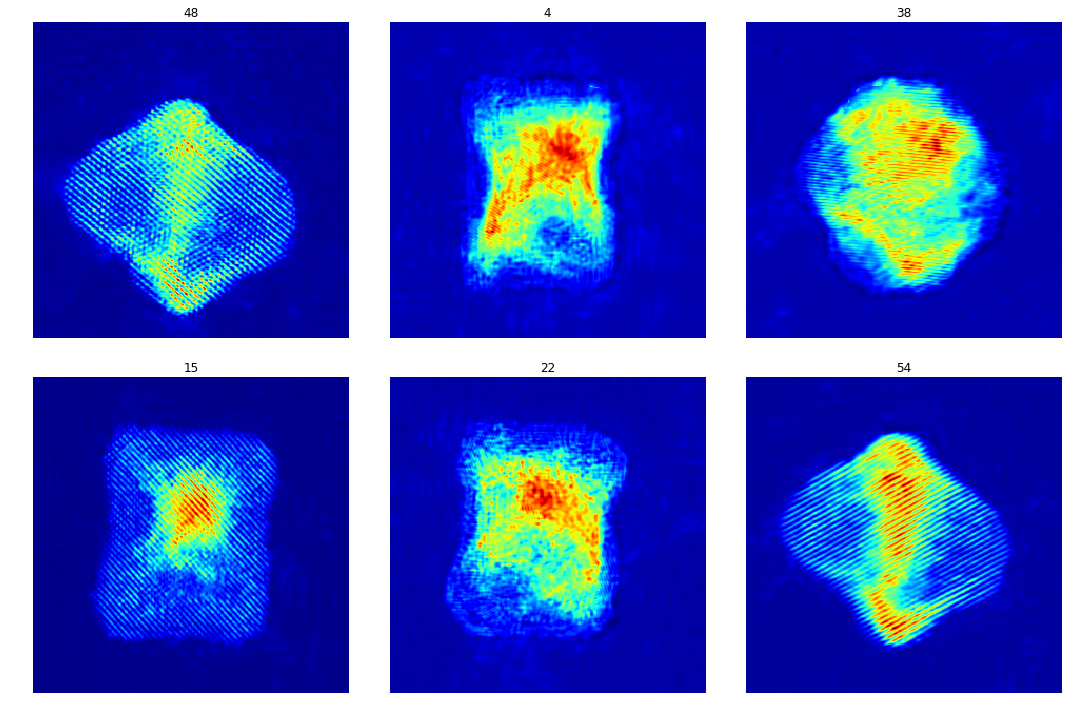
The train model is tested on 60 experimental images.

test_raw = sio.loadmat('./data_aet/Raw/NiPt_Mo_FS_171118_t2_BM3D100_results.mat')
test_raw = test_raw['Dset']
plt.figure(figsize=(15,10))
c = 1
idx = np.random.randint(1, test_raw.shape[2], 6)
for i in idx:
    plt.subplot(2,3,c)
    plt.imshow(test_raw[:,:,i], cmap='jet')
    plt.axis('off')
    plt.title(i)
    plt.tight_layout()    
    c += 1    

test_res = sio.loadmat('./results/exp/NiPt_Mo_DnCNN_predictions.mat')
test_res = test_res['img_new']
plt.figure(figsize=(15,10))
c = 1
for i in idx:
    plt.subplot(2,3,c)
    plt.imshow(test_res[:,:,i], cmap='jet')
    plt.axis('off')
    plt.title(i)
    plt.tight_layout()
    c += 1  

Conclusion

I adapted a deep learning denoising framework (DnCNN) for doing background subtraction in atomic electron tomography preprocessing. The idea is that such supervised, discriminative learning can be part of a general data preprocessing pipeline for tomography reconstruction.

Future improvements

• This model is trained on pretty basic estimation of background (Gaussian). A more sophisticated model of the background can help train better model
• Train images with different features separately can maybe enhance training quality. Some projection images taken along zone axis contains much